Activation Functions: How Simple Curves Power Neural Networks

Source: Dev.to

Activation Functions – The Building Blocks of Neural Networks

In my previous article we touched upon the sequence‑to‑sequence model and introduced RNNs (Recurrent Neural Networks).
To understand RNNs we first need to understand the basics of neural networks, starting with activation functions.

What is an activation function?

A neural network is composed of layers, each containing many neurons. Inside a neuron two things happen:

1. Inputs are combined using weights.
2. The result is passed through an activation function.

Think of the activation function as a weighing scale – it decides how much a neuron should fire for a given input.

Activation functions as curves

Activation functions are mathematical curves that transform input values into output values. The most commonly discussed ones are:

• ReLU
• Softplus
• Sigmoid

Below we’ll use a tiny Python snippet (NumPy + Matplotlib) to visualise each function.

import numpy as np
import matplotlib.pyplot as plt

Generating input values

# 400 evenly spaced values from -10 to 10
x = np.linspace(-10, 10, 400)

• -10 → start of the range (most negative input)
• 10 → end of the range (most positive input)
• 400 → number of points, giving a smooth curve when plotted

x represents the inputs to the activation functions. By passing all these values through a function (e.g., ReLU or Sigmoid) we can visualise how the function transforms inputs to outputs.

1. ReLU (Rectified Linear Unit)

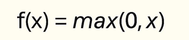
• If the input is negative, the output is 0.
• If the input is positive, the output is the same value.

def relu(x):
    return np.maximum(0, x)

plt.figure()
plt.plot(x, relu(x), label="ReLU")
plt.title("ReLU Activation Function")
plt.xlabel("Input")
plt.ylabel("Output")
plt.grid(True)
plt.legend()
plt.show()

ReLU is the default choice for most modern neural networks because of its simplicity and efficiency.

2. Softplus (Smooth ReLU)

Softplus is a smooth version of ReLU. Where ReLU has a sharp corner at zero, Softplus transitions gradually.

def softplus(x):
    return np.log(1 + np.exp(x))

plt.figure()
plt.plot(x, softplus(x), label="Softplus")
plt.title("Softplus Activation Function")
plt.xlabel("Input")
plt.ylabel("Output")
plt.grid(True)
plt.legend()
plt.show()

Softplus avoids the “dead neuron” problem of ReLU, but it is computationally more expensive, so it’s used less often in practice.

3. Sigmoid

The sigmoid squashes any input into the interval (0, 1), making it useful for binary‑classification outputs.

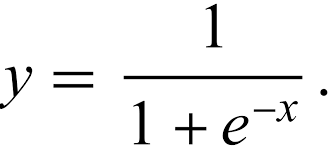
def sigmoid(x):
    return 1 / (1 + np.exp(-x))

plt.figure()
plt.plot(x, sigmoid(x), label="Sigmoid")
plt.title("Sigmoid Activation Function")
plt.xlabel("Input")
plt.ylabel("Output")
plt.grid(True)
plt.legend()
plt.show()

The output is an S‑shaped curve, ideal for binary‑classification outputs.

Take‑away

• ReLU – simple, fast, default for hidden layers.
• Softplus – smooth version of ReLU, mitigates sharp‑corner issues at a higher computational cost.
• Sigmoid – maps to (0, 1), ideal for output layers in binary classification but suffers from vanishing gradients in deep networks.

Understanding these activation functions is the first step toward mastering more complex architectures such as RNNs and sequence‑to‑sequence models. Happy coding!

You can try the examples out via the Colab notebook.

---

Just like activation functions make neurons work efficiently in a network, having the right tools can make your work as a developer much easier. If you’ve ever struggled with repetitive tasks, obscure commands, or debugging headaches, this platform is here to make your life easier. It’s free, open‑source, and built with developers in mind.

Explore the platform →