Image Classification with CNNs – Part 3: Understanding Max Pooling and Results

Source: Dev.to

Max Pooling

In the previous article we created a feature map.
Now we apply another filter to that feature map.
Instead of computing a dot product, the filter selects the maximum value in each region and moves so that it does not overlap itself.

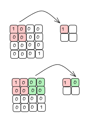
When we take the maximum value from each region we are performing max pooling.
Max pooling keeps the regions where the filter best matches the input image.

---

Average Pooling

Alternatively, we can compute the average (mean) value for each region. This operation is called average pooling (or mean pooling).

---

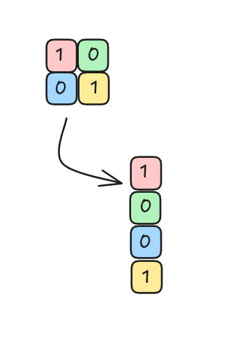
Flattening the Pooled Layer

After pooling, the resulting feature map is reshaped into a column of input nodes (a flattened vector) that can be fed into a fully‑connected network.

---

Fully Connected Neural Network

The flattened vector is connected to a fully connected neural network:

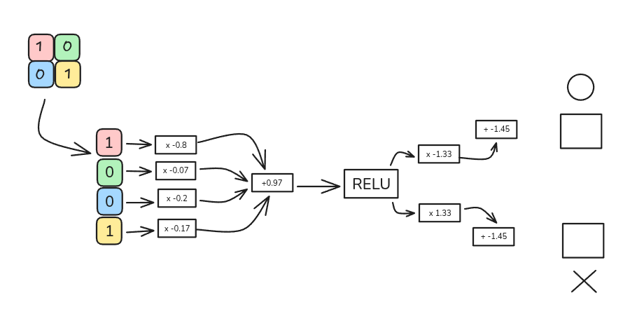
The network architecture used in this example:

• 4 input nodes (one for each element of the flattened vector)
• One hidden layer with a ReLU activation function
• 2 output nodes, representing the letters O and X

Example Calculation

1. Weighted sum for a hidden node

   [ (1 \times -0.8) + (0 \times -0.07) + (0 \times 0.2) + (1 \times 0.17) = -0.63 ]

2. Add bias

   [ -0.63 + 0.97 = 0.34 ]

   The input to the ReLU activation function is 0.34.

3. Apply ReLU

   [ \text{ReLU}(0.34) = \max(0, 0.34) = 0.34 ]

4. Output layer

   • For the letter O, after multiplying by the output weights and adding the bias, the result is 1.
   • For the letter X, the result is 0.

Thus, when the input image is the letter O, the network correctly classifies it as O.
The same process can be repeated for the letter X, which will be covered in the next article.