Cross Entropy Derivatives, Part 6: Using gradient descent to reach the final result
Source: Dev.to
Optimizing the Bias (b_3) – Getting the Exact Value
In the previous article we plotted a curve that helps us optimise the bias.
In this article we compute the accurate value for (b_3).
Derivative of the Cross‑Entropy Loss w.r.t. (b_3)
Because we have three observations and make one prediction per observation, the total derivative is obtained by summing one term per prediction.
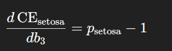
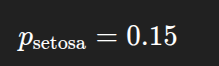
1️⃣ First Observation
We focus on the prediction for the first observation.
The observed species is Setosa, so we compute the cross‑entropy using the predicted probability for Setosa.
The network’s forward‑pass expression (from the previous article) is:
For petal width = 0.04 and sepal width = 0.42, the predicted probability for Setosa is:
Hence the contribution from the first observation to the derivative is
[ \frac{\partial L_1}{\partial b_3}= \hat{y}_1 - y_1 = 0.15 - 1 . ]
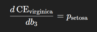
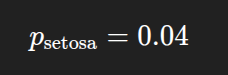
2️⃣ Second Observation
The second observation belongs to the species Virginica.
The derivative term for this observation is:
Using petal width = 1.0 and sepal width = 0.54, the predicted probability for Setosa is:
3️⃣ Third Observation
The third observation belongs to the species Versicolor, so the derivative term is again:
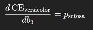
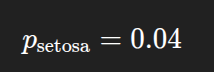
For petal width = 0.50 and sepal width = 0.37, the predicted probability for Setosa is:
📐 Total Derivative
Adding the three contributions:
[ \begin{aligned} \frac{\partial L}{\partial b_3} &= (0.15 - 1) ;+; 0.04 ;+; 0.04 \ &= -0.77 . \end{aligned} ]
This value represents the slope of the tangent line to the loss curve at (b_3 = -2).
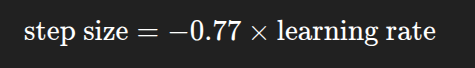
🔄 Gradient‑Descent Update
We now plug this slope into the gradient‑descent update rule:
[ b_3^{\text{new}} = b_3^{\text{old}} - \alpha \frac{\partial L}{\partial b_3} ]
If we set the learning rate (\alpha = 1), then
[ b_3^{\text{new}} = -2 - ( -0.77 ) = -2 + 0.77 = -1.23 . ]
The update step is visualised as:
We repeat this process, using the updated value of (b_3) each time, until one of the stopping criteria is met (predictions stop improving, a maximum number of steps is reached, etc.).
In this example the predictions stop improving when (b_3 = -0.03).
🚀 Looking for an easier way to install tools, libraries, or entire repositories?
Try Installerpedia – a community‑driven, structured installation platform that lets you install almost anything with minimal hassle and clear, reliable guidance.
ipm install repo-name…and you’re done! 🎉
End of article.