Schemas & Data Modelling in Power BI

Source: Dev.to

Data modelling is the process of structuring your tables and defining relationships so Power BI can:

• Aggregate data correctly
• Filter data efficiently
• Produce accurate measures
• Perform fast, even with large datasets

Think of it as designing the blueprint of your report before decorating it with visuals.

Star Schema Overview

Star schema is a mature modelling approach widely adopted by relational data warehouses.
It requires modelers to classify their model tables as either dimension or fact.

Dimension Tables

Dimension tables describe business entities—the things you model.
Entities can include products, people, places, concepts, and even time itself.

• A dimension table contains a key column (or columns) that acts as a unique identifier, plus additional columns that support filtering and grouping.
• The most consistent table in a star schema is the date dimension table.

Fact Tables

Fact tables store observations or events (e.g., sales orders, stock balances, exchange rates, temperatures).

• A fact table contains dimension key columns that relate to dimension tables and numeric measure columns.
• The dimension key columns determine the dimensionality of a fact table, while the key values determine its granularity.

Example – A fact table that stores sales targets has two dimension key columns: Date and ProductKey.

• The table has two dimensions (Date and Product).
• If the Date column stores the first day of each month, the granularity is month‑product level.

Generally, dimension tables contain a relatively small number of rows, whereas fact tables can contain many rows and continue to grow over time.

Fig. 1.1 – Star schema layout

Normalization vs. Denormalization

To understand star‑schema concepts, it’s important to know two terms:

• Normalization – Storing data to reduce repetition.
  Example: a product table with a unique ProductKey and descriptive columns (name, category, color, size). A sales table that stores only the ProductKey is normalized.

  
  Fig. 1.2 – Normalized sales table (only ProductKey)

• Denormalization – Storing redundant data for convenience or performance.
  Example: a sales table that also includes product name, category, etc.

  
  Fig. 1.3 – Denormalized sales table (ProductKey + product attributes)

When you source data from an export file or data extract, it’s often already denormalized. Use Power Query to transform and shape the source into multiple normalized tables.

Note: While you should aim for normalized fact and dimension tables, a snowflake dimension may be deliberately denormalized to produce a single model table.

Star Schema Relevance to Power BI Semantic Models

Star‑schema design and the concepts above are highly relevant to building Power BI models that are both performant and user‑friendly.

• Each Power BI visual generates a query against the semantic model.
• Queries typically filter, group, and summarize data.

A well‑designed model therefore provides:

• Dimension tables for filtering and grouping.
• Fact tables for summarization.

There is no explicit property to label a table as “dimension” or “fact.” The role is inferred from model relationships:

• The cardinality of a relationship (one‑to‑many or many‑to‑one) determines the table type.
• The “one” side is always a dimension table; the “many” side is always a fact table.

Fig. 1.4 – One‑to‑many relationship (dimension → fact)

Snowflake Dimension

A snowflake dimension is a set of normalized tables that represent a single business entity.
For example, in the Adventure Works data warehouse, products are classified by category and subcategory:

• A product belongs to a subcategory.
• A subcategory belongs to a category.

The product dimension is therefore stored in three related, normalized tables.

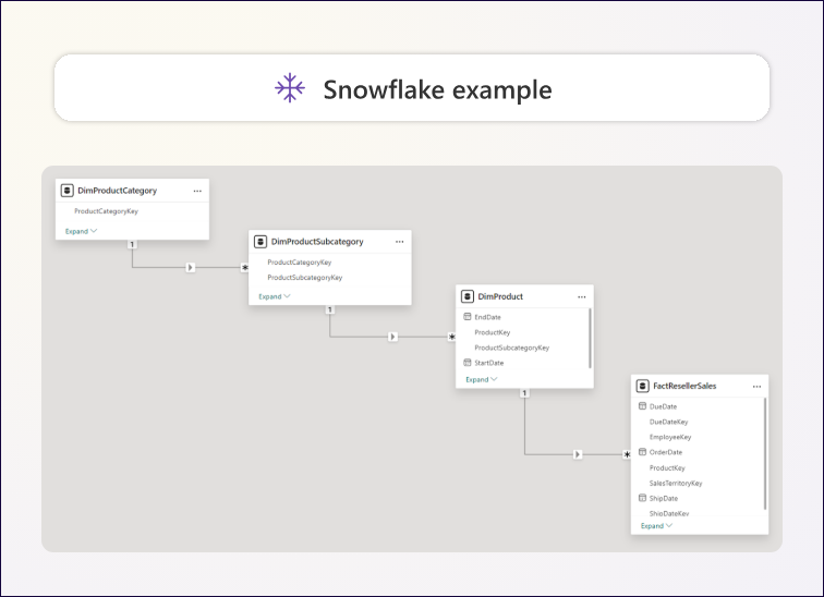
Fig. 1.5 – Normalized tables for the product dimension.

If you picture the normalized tables radiating outward from the fact table, you can see the classic “snowflake” shape.

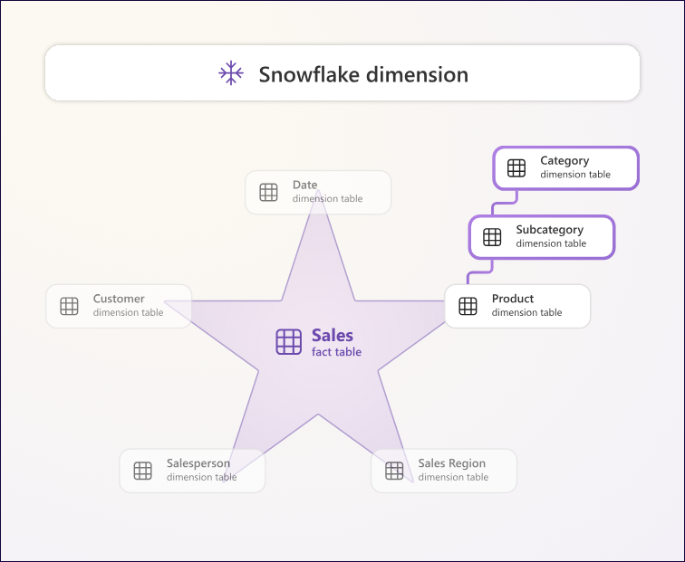
Fig. 1.6 – Snowflake design illustration.

Snowflake vs. Denormalized Design in Power BI Desktop

In Power BI Desktop you can either:

1. Mimic a snowflake dimension design (often because the source data is already normalized), or
2. Combine the source tables into a single, denormalized model table.

Generally, a single model table provides more benefits, but the optimal choice depends on data volume and usability requirements.

When you mimic a snowflake dimension design

• Storage & performance: More tables are loaded, which can be less efficient. Each table must contain columns to support relationships, increasing model size.
• Filter propagation: Longer relationship chains must be traversed, potentially reducing filter efficiency.
• User experience: The Data pane shows many tables, which can be confusing—especially when snowflake tables contain only one or two columns.
• Hierarchies: You cannot create a hierarchy that spans columns from multiple tables.

When you integrate into a single model table

• Hierarchies: You can define a hierarchy that covers the full grain of the dimension (from highest to lowest level).
• Storage impact: Redundant, denormalized data may increase model size, particularly for large dimension tables.

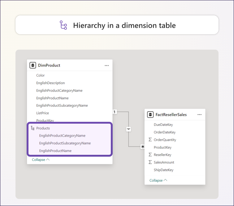
Fig. 1.7 – Comparison of snowflake and denormalized designs in Power BI.

Key Takeaway

Choose the design that balances performance, storage, and user experience for your specific scenario. Snowflake designs can be useful when source data is already normalized, but a well‑designed denormalized model often yields better performance and a more intuitive reporting experience.