Building Elbow Arrows in Excalidraw (Part 2)

Source: Dev.to

Previously on Building Elbow Arrows…

In part one we identified the design goals (shortest route, minimal segments, proper arrow orientation and shape avoidance), but our naive and greedy first approach to the algorithm turned out to be inadequate on multiple fronts. Therefore this approach is abandoned in favor of a different algorithm.

Games to the Rescue

The design goals were suspiciously similar to the problem of path‑finding in video games, which is a common, well‑researched problem. Characters in these games often have to find their way from point A to point B on the game map, without getting blocked by obstacles, and use the shortest route. They also need to make it look like a human would take that route, so these characters don’t break immersion. Thus, we turn our focus to the A* search algorithm.

Building the Foundations

To understand A* path‑finding we need to understand the context, some of the other graph‑search algorithms it is built on and improved from, and how they can help solve our challenge.

• Where A* comes from – It is part of a family of algorithms for graph search, all of which aim to find the shortest path in a graph of nodes connected by edges. While this makes them useful far beyond just games, we’ll focus on path‑finding in a 2D grid (i.e. the canvas).
• Turning the canvas into a graph – If we split the canvas into a 2D grid (at the extreme, every pixel is its own cell), the neighboring (common) sides of each pair of cells can be represented by edges of a graph where the nodes are the cells themselves.

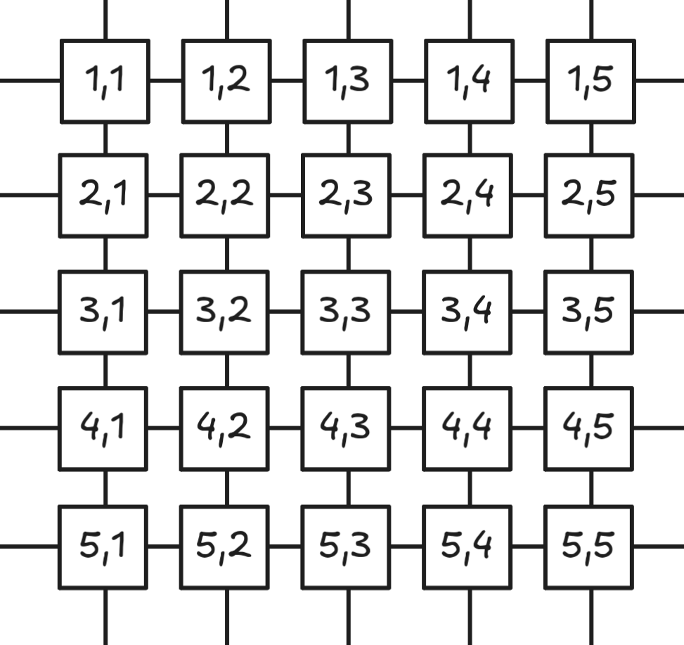
If we can find a route across these node edges (grid cells) satisfying our original constraints, we can simply draw the elbow arrow itself!

Breadth‑First Search

One simple graph‑search algorithm that guarantees the shortest path in an unweighted graph is the humble Breadth‑First Search (BFS), which is where we will start our exploration.

• BFS visits all directly connected, unvisited nodes from already visited nodes in each iteration (starting with the start cell).
• It continues until the cell containing the end point is visited.
• While exploring, we record which adjacent node we came from for every visited node, forming a linked list back toward the start node.
• When we reach the end point (we can exit early because the path is optimal), we backtrack through that list to obtain the shortest path.

The resulting path is the shortest possible, but it does not look like an elbow arrow and is therefore not visually pleasing. It is, however, a solid foundation on which we can build.

NOTE: If you’re interested in diving deeper into BFS, DFS, and how A* works, I recommend this article, which dives deeper into these algorithms and offers interactive visualizations. This guide will only cover the key insights needed for the final elbow‑arrow implementation.

Dijkstra’s Algorithm

BFS gives us the shortest path and avoids obstacles, but it still doesn’t produce the orthogonal bends we need for an elbow arrow. To encourage the algorithm to take the desired shape, we turn to Dijkstra’s algorithm.

• Dijkstra operates on weighted graph edges, using the weights as the cost to visit a neighbor.
• Imagine the canvas has a third “depth” dimension: cells that lie on a correct elbow‑arrow route are flat, while all other cells are steep “walls”.
• Our “maze generator” can then assign low costs (valleys) to cells that satisfy the design goals and high (or prohibitive) costs to everything else.

Because the Excalidraw canvas is effectively infinite, we cannot pre‑compute the entire terrain. Instead, the algorithm must be able to query, for any given cell, which neighboring cells are cheap to visit and which are expensive.

Distance Functions

The key to shaping the terrain is a well‑chosen distance function. Edge weights should naturally decrease toward the end cell, creating a downward “slope” (a negative gradient) while making incorrect choices expensive.

• Euclidean distance – the straight‑line length between two points.
• Manhattan (Taxicab) distance – more appropriate for our orthogonal arrow routes. It is calculated by adding the absolute differences of the coordinates:

[ \text{Manhattan}(p_1, p_2) = |x_1 - x_2| + |y_1 - y_2| ]

For example, the distance between ([5, 12]) and ([10, -3]) is (|5-10| + |12-(-3)| = 5 + 15 = 20).

The illustration below shows a Euclidean (green) line and three equal‑length Manhattan paths (red, blue, and yellow).

Using Manhattan distance as the heuristic for A* (or as the weight function for Dijkstra) encourages the algorithm to favor orthogonal moves, giving us the characteristic elbow‑arrow shape we desire.

Additional Heuristics

Querying the Manhattan distance at every cell we want to visit in our Dijkstra algorithm gives us a metric we can use to generate the maze for our search algorithm, but it offers multiple equally‑weighted paths and we need to choose the one with the shortest amount of orthogonal bends.

We add an additional term to our maze generator: we not only consider the Manhattan distance of a neighboring cell to the end cell, but we also increase the cost of a neighbor if moving to it would create a bend in the path.

Search metric:

Manhattan distance + bend count

This weighting function, paired with Dijkstra’s algorithm, now generates correct, visually‑pleasing elbow arrows when there are no obstacles to avoid.

Exclusion Zones

To support shape avoidance we need to deactivate some cells. These cells behave like infinitely high walls in our maze, so the graph‑search algorithm never visits them. This is easily achieved by adding a flag to every cell, mapping shapes to those cells, and disabling the cells covered by the shapes.

However, combined with our modified distance calculation, the algorithm starts to take sub‑optimal paths around shapes. The reason is that we can’t see the entire “map” (i.e. the grid); it’s like a fog of war that we uncover at each iteration of the search. Obstacles we should avoid well in advance might not be “seen” until it’s too late.

Introducing a back‑tracking process is one practical way to address this, but it can be computationally infeasible. To reduce unnecessary exploration steps and incorporate our heuristics, the A* algorithm seemed like an optimal choice.

A* is similar to Dijkstra’s algorithm—it considers the weight of graph edges—but it prioritizes exploring those neighboring nodes (or cells) that offer the best chance of moving closer to the goal, thereby avoiding wasted computation. It also promises a one‑pass solution that is memory‑efficient.

What is A*?

The key insight of A* is that it balances two factors for every cell (node):

• g(n) – the actual cost to reach a node from the start (our bend count plus any additional heuristics later).
• h(n) – the estimated cost to reach the goal from that node (Manhattan distance + grid exclusion + any extra heuristic functions).
• f(n) = g(n) + h(n) – the total estimated cost of the path through that node.

The algorithm maintains two sets of nodes:

• Open set – nodes to be evaluated.
• Closed set – nodes already evaluated.

Process

1. Add the start node to the open set.
2. Loop until the open set is empty:
   • Select the node with the lowest f(n) score.
   • If it’s the goal, reconstruct the path and return it.
   • Move the node to the closed set.
   • For each neighbor:
     • Calculate a tentative g score.
     • If the neighbor is in the closed set and the new g score is worse, skip it.
     • If the neighbor isn’t in the open set or the new g score is better:
       • Update the neighbor’s scores.
       • Set the current node as the neighbor’s parent.
       • Add the neighbor to the open set.
3. If the open set becomes empty without finding the goal, no path exists.

By always exploring the node with the lowest f(n) value, A* efficiently finds optimal paths without exhaustively searching every possibility—exactly what we want. At this stage the implementation mostly worked as expected, but edge cases kept popping up where a human would expect a different routing choice, and performance was still an issue.

Performance Optimizations

While the behavior was close, performance quickly became a bottleneck, especially when multiple elbow‑arrow paths had to be calculated for every frame. Targeting at least 120 Hz smooth rendering with ~50 elbow arrows re‑routing each frame was a lofty, but achievable, goal.

Binary Heap Optimization

The low‑hanging fruit was the open set of nodes (cells). Performing a linear lookup across open nodes at every iteration is not ideal. The obvious cure is to store the open set in a binary heap, giving us O(log n) insertion and removal instead of O(n).

Non‑Uniform Grid

Operating on a pixel‑grid (one node per pixel) causes a massive number of unnecessary A* iterations (often > 99 %). Even using cells that span just a few pixels wastes a lot of work and prevents pixel‑perfect results.

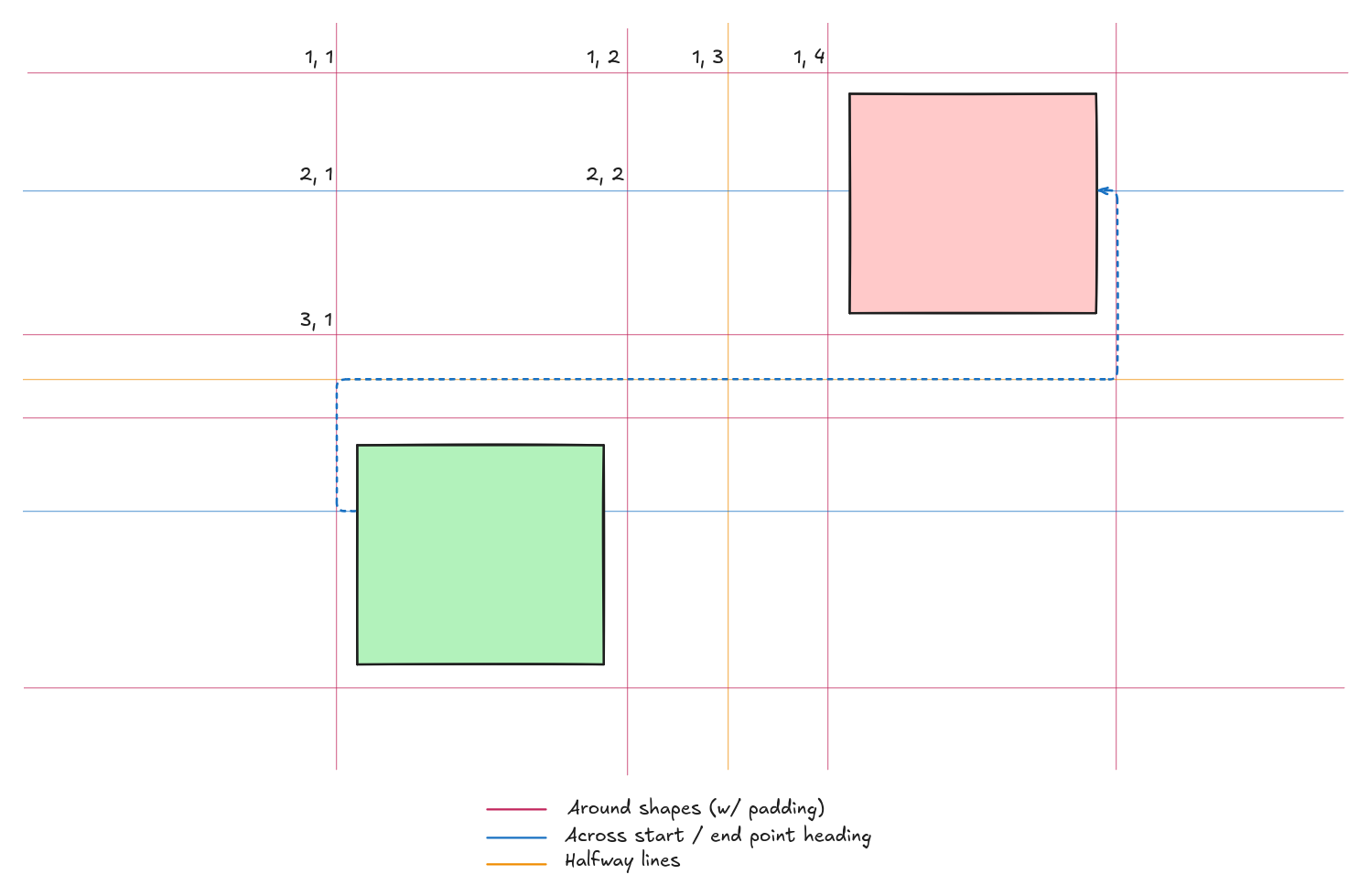
The solution is to draw a non‑uniform grid that only places nodes where a potential bend could occur. Aesthetically pleasing elbow arrows always break at:

• Shape corners,
• Start and end point headings,
• Mid‑points between shapes to be avoided (with optional padding).

Because the algorithm works on graph nodes, nothing forces us to use a uniformly‑sized grid. The only requirement for A* and the Manhattan‑distance calculation is that neighboring cells have contiguous Cartesian coordinates.

Adaptive Grid (preview)

The article continues with an exploration of how to dynamically generate and adapt the non‑uniform grid based on the current layout of shapes, but the excerpt ends here.

Image credit: Wikipedia (via dev.to)

A* with Manhattan Distances for Aesthetic and Performant Elbow Arrows

Aesthetic Heuristics

While the basic A* implementation produced better results than the BFS approach, there were still cases—beyond the excessive bend count—that generated unnatural routes. By carefully constructing additional heuristics we were able to address these issues. However, changes to the A* metric affect all edge cases, so testing and fine‑tuning were done manually to arrive at the final solution.

1. Backward Visit Prevention

Arrow segments are prohibited from moving backwards (i.e., overlapping with previous segments) when there is no alternative route. This not only prevents spike‑like paths (directly reversed segments) but also almost completely avoids routes that would require a U‑shaped arrow configuration.

• How it works
  • Track the direction of visits.
  • Look back one step and forward one step to detect the problematic configuration.
  • Combine this with a very specific grid selection to prevent the edge cases where the issue would otherwise trigger.

Note: This works because there can be at most two closed axis‑aligned bounding boxes (the shapes) to avoid. With more obstacles the problem would re‑appear.

2. Segment Length Consideration

Longer straight segments (in Euclidean distance) are preferred over multiple short segments, even though Manhattan distance is the primary metric driving the A* pathfinding. In some edge cases the non‑uniform grid assumes a generated path is the shortest, but when projected onto the pixel grid it creates short‑step patterns that should not exist—especially when connected shapes are far apart.

3. Shape‑Side Awareness

When choosing whether to route left or right around an obstacle, the algorithm considers:

• The length of the obstacle’s sides.
• The relative position of the start and end points heading‑wise (see “heading” in part 1 of this series).
• The parallel or orthogonal relationship between the arrow and the shape’s bounding‑box side.

4. Short Arrow Handling

Special logic handles cases where the start and end points are extremely close. This prevents excessive meandering and loops. In one scenario where connected shapes almost overlap, a hard‑coded simplified direct route is used because the expected route would never emerge from the generic algorithm.

5. Overlap Management

The implementation explicitly detects when shapes cover the start and/or end points. When connected shapes or points overlap, it selectively disables avoidance for one shape or both, ensuring a valid route exists even if the exclusion zones would otherwise block it.

Other Solutions

Using A* with Manhattan distances is not the only way to obtain orthogonal (elbow) arrows. Below are some research papers that were considered but ultimately not adopted:

• Gladisch, V., Weigandt, H., Schumann, C., & Tominski, C.
  Orthogonal Edge Routing for the EditLens – arXiv:1612.05064

• Wybrow, M., Marriott, K., & Stuckey, P. J.
  Orthogonal Connector Routing – Springer PDF

Conclusion

What began as a simple feature request—“add elbow arrows”—evolved into a sophisticated path‑finding challenge. By combining:

• Classical algorithms (A*),
• Domain‑specific optimizations (non‑uniform grids, only two shapes to avoid, etc.), and
• Carefully tuned heuristics (aesthetic weights),

Excalidraw’s elbow arrows dramatically speed up diagramming and eliminate the need for hand‑drawn, hand‑managed arrows.

These improvements also enabled other powerful features, such as keyboard‑shortcut flowchart creation (watch the demo), further empowering Excalidraw users with serious diagramming needs.

Next up: Join me for the third and final part of this series on elbow arrows, where I walk you through how controlling and fixing arrow segments makes difficult‑to‑predict routes possible for power users!